Capital Asset Pricing Model for IBM Stocks

Analysis of IBM’s 1994-2015 stock market performance using Capital Asset Pricing Model (CAPM).

Step 1: Imported the data into RStudio environment

The data contains:

• Dates (Jan 1994 - Dec 2015)
• IBM’s daily return
• Market’s daily return
• Daily risk-free rate

Step 2: Computed yearly excess market and IBM stock returns

lg <- length(ibmRET)
IBMEXRET_Annualized <- rep(NA,lg)
marketEXRET_Annualized <- rep(NA,lg)

for (i in 252:lg){
  IBMEXRET_Annualized[i] <- (prod(IBMEXRET[(i-252+1):(i)]/100+1)-1)*100 # Daily excess IBM returns
  marketEXRET_Annualized[i] <- (prod(marketEXRET[(i-252+1):(i)]/100+1)-1)*100 # Daily excess Market Returns
} 

Time-series plot of market’s annual excess return:

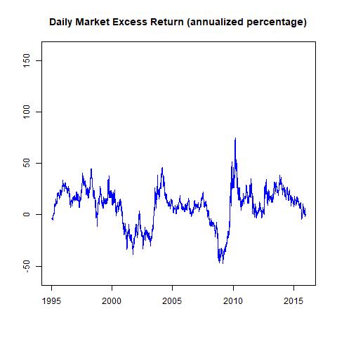
Step 3: Found the global maximum

On 3rd September 2010, the market was at the global maximum (75.06%).

Step 4: Computed 5-yearly excess market and IBM stock returns

IBMEXRET_5Year <- rep(NA,lg)
marketEXRET_5Year <- rep(NA,lg)

for(i in (252*5):lg){
  IBMEXRET_5Year[i] <- (prod(IBMEXRET[(i-252*5+1):(i)]/100+1)^(1/5)-1)*100 # Five-year IBM excess returns
  marketEXRET_5Year[i] <- (prod(marketEXRET[(i-252*5+1):(i)]/100+1)^(1/5)-1)*100 # Five-year Market excess returns
}

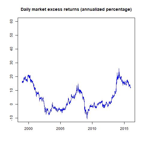
Time-series plot of market’s 5-yearly excess return:

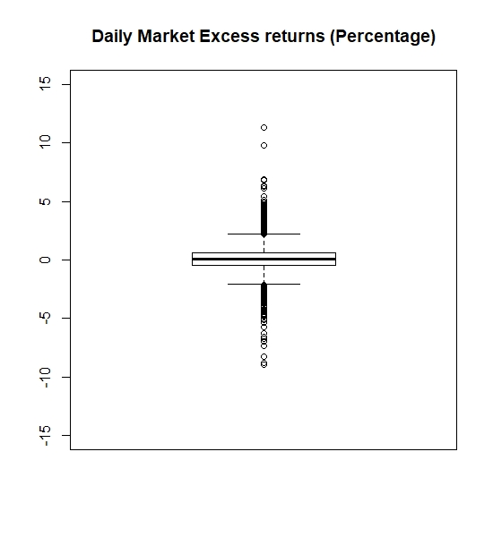
Step 5: Visualize the spread of the daily returns

• Boxplot of excess market returns:

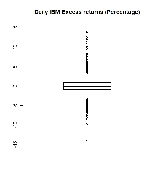
• Boxplot of excess IBM’s stock returns:

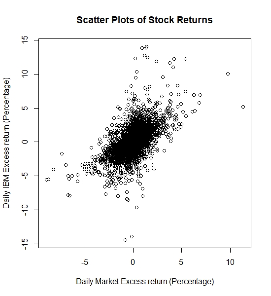
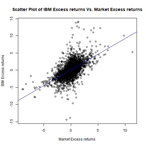
• Scatter-plot of daily IBM vs. market excess returns:

Step 6: Check the various moments of IBM’s and market excess returns:

Metric	IBM’s daily stock return	Market’s daily stock return
Mean	17.38198%	7.892513%
Standard deviation	28.8362%	18.83606%
Skewness	0.580013	-0.1168607
Kurtosis	8.060213	7.639527
Minimum	-14.41947%	-8.95%
Maximum	14.05134%	11.35%
Sharpe ratio	0.6028	0.4190
Value at Risk	-2.6330%	-1.8305%
Expected Shortfall	-3.9803	-2.8095
Correlation	0.5956	NA

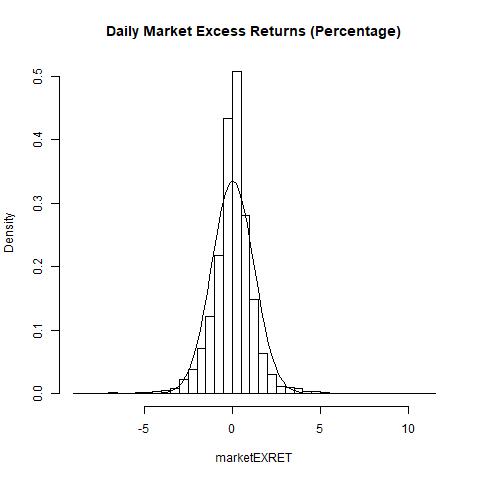
Histogram of market’s excess returns:

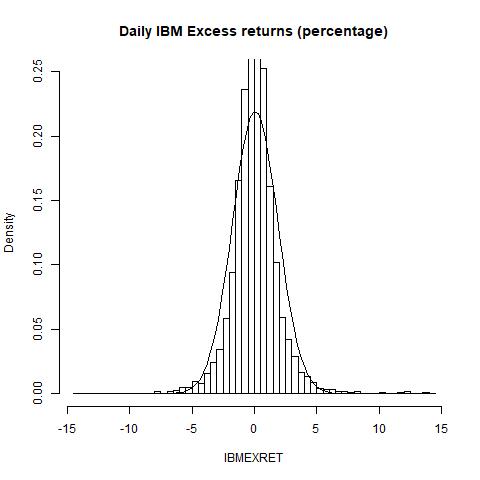
Histogram of IBM’s excess returns:

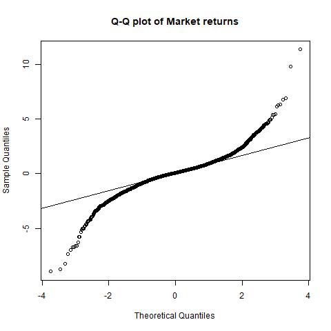
QQ-plot for market’s excess returns:

QQ-plot for IBM’s excess returns:

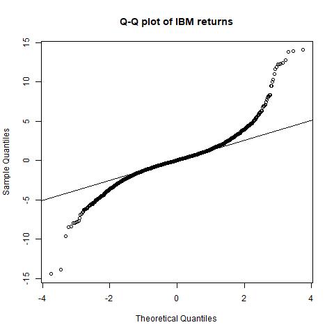
Step 7: Hypothesis testing

1. The Jarque-Bera Test:
   • For IBM: X-squared = 15322, degrees of freedom = 2, p-value < 2.2e-16
   • For market: X-squared = 13498, degrees of freedom = 2, p-value < 2.2e-16
2. The Lilliefors Test:
   • For IBM: D = 0.081205, p-value < 2.2e-16
   • For market: D = 0.084228, p-value < 2.2e-16

Step 8: Linear model estimation

We try to explain the behavior of IBM’s returns through market’s returns.

Results:

1. Residuals:

Min	1Q	Median	3Q	Max
-13.8015	-0.6594	-0.0582	0.5996	12.9184

1. Coefficients:

Coefficient	Estimate	Std. Error	t value	Pr > t
(Intercept)	0.04042	0.01961	2.061	0.0394
marketEXRET	0.91177	0.01653	55.175	<2e-16

Residual standard error: 1.459 on 5538 degrees of freedom

Multiple R-squared: 0.3547, Adjusted R-squared: 0.3546

F-statistic: 3044 on 1 and 5538 DF, p-value: < 2.2e-16

Plot of OLS line:

Alternate hypothesis: Is the risk adjusted returns zero? Result: Cannot reject null hypothesis, so risk-adjusted returns are not zero!

Note:

• Sharpe ratio:

• Value at Risk (VaR):

• Expected Shortfall: , where is the confidence level